In this article, you will explore how JAX can be used as a Deep Learning Framework and discuss its advantages and disadvantages compared to other popular frameworks.
A Zero to Advanced Guide on JAX
In today’s world AI is the most trending topic and most talked about. With the introduction of Generative AI, many developers and hardware engineers have tried to build AI applications. So learning Machine Learning and Deep Learning algorithms is the starting point in the World of AI. But building such Machine Learning and Deep Learning algorithms is not easy.
Thus we have many Deep Learning frameworks that will make this task easier. The most popular Deep Learning Frameworks include TensorFlow, PyTorch, and JAX. JAX offers a unique combination of performance, ease of use, and flexibility.
What is JAX and why is it growing in popularity?

JAX (short for “Just-in-time” Accelerated X) is a relatively new Python library developed by Deepmind that gained popularity in the machine learning and research communities. Further it enables high-performance numerical computing while also being easy to use and flexible. It is built on top of the Python language and has become increasingly popular due to its ability to automatically differentiate functions using a technique called Automatic differentiation. Also referred to as Auto Grad.
One of the main reasons why JAX has become popular in recent years is its compatibility with NumPy. This compatibility allows developers to easily switch between these libraries without having to rewrite their code from scratch. Additionally, it has several features that make it well-suited for research, including support for higher-order functions, composable function transformations, and a functional programming style that encourages modularity and abstraction.
Installation
JAX is written in Python, but it depends on XLA, which needs to be installed as the jaxlib package.
For CPU:
pip install --upgrade "jax[cpu]" -f https://storage.googleapis.com/jax-releases/jax_releases.html
For Cuda:
pip install --upgrade "jax[cuda]" -f https://storage.googleapis.com/jax-releases/jax_releases.html
JAX Quickstart: Let’s Implement JAX
JAX is a powerful and flexible Machine Learning framework that allows for high-performance computing on both CPUs and GPUs. By following these quickstart guides, you’ll learn how to build and train ML models using JAX and gain a deeper understanding of the principles and techniques involved.
import numpy as np
import matplotlib.pyplot as plt
import jax.numpy as jnp
Numpy vs JAX
The syntax of JAX is similar to Numpy, and thus it is often referred to as “Numpy for GPU”. We will see that in the later part of this article.
X = np.linspace(0,20,10000)
sin_func = np.sin(X)
cos_func = np.cos(X)
plt.plot(X, sin_func,label="sin")
plt.plot(X,cos_func,label="cos")
plt.legend()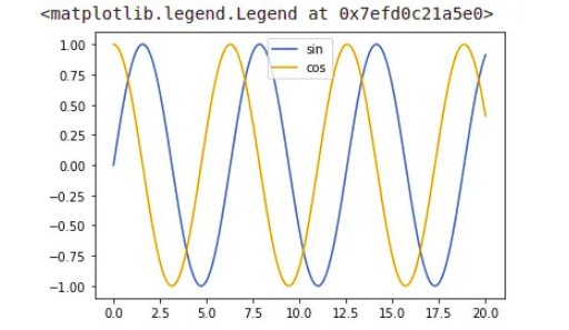
X_jax = jnp.linspace(0, 20, 1000)
sin_jax = jnp.sin(X_jax)
cos_jax = jnp.cos(X_jax)
plt.plot(X_jax, sin_jax,label="sin")
plt.plot(X_jax,cos_jax,label="cos")
plt.legend()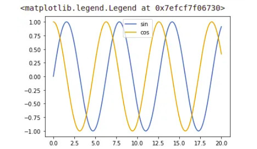
The above code is running on GPU runtime in Google Colab, as mentioned earlier, JAX is Numpy for GPU, the JAX code will detect whether the code has been executed on GPU/TPU or not. If it is running on CPU runtime, then it will display a message “No GPU/TPU found, falling back to CPU. (Set TF_CPP_MIN_LOG_LEVEL=0 and rerun for more info.)”.
arr_numpy = np.arange(10)
arr_jax = jnp.arange(10)

print(arr_numpy)
print(arr_jax)

#Output:
#[0 1 2 3 4 5 6 7 8 9]
#[0 1 2 3 4 5 6 7 8 9]

arr_numpy[0] = 1 #Mutable
arr_jax[0] = 4 #error:  JAX arrays are immutable.
Numpy arrays are mutable, whereas Jax arrays are immutable.
Random numbers
Pseudorandom number generators (PRNGs) from libraries like NumPy abstract away the underlying details and provide a convenient source of pseudorandomness, allowing users to easily generate sequences of seemingly random numbers. Underneath the hood, numpy uses the Mersenne Twister PRNG to power its pseudorandom functions. The PRNG has a period of 219937−1.
print(np.random.random())JAX uses an explicit pseudorandom number generator (PRNG) that requires the user to explicitly pass and iterate the PRNG state for entropy production and consumption.
from jax import random
key = random.PRNGKey(0)
print(random.normal(key, shape=(1,)))
Basic JAX operations
arr1 = jnp.array([1,2,3])
arr2 = jnp.array([4,5,6])
result1 = jnp.add(arr1,arr2)
result2 = jnp.subtract(arr1,arr2)
result3 = jnp.dot(arr1,arr2)

print("Add:",result1)
print("Sub:",result2)
print("Dot:",result3)

#Output
#Add: [5 7 9]
#Sub: [-3 -3 -3]
#Dot: 32
Convolve Operation
The convolve operation is used to combine these two functions to produce a third function.
x = jnp.array([1, 2, 1]) #x is an array of length 3
y = jnp.ones(10) # y is an array of length 10 filled with ones.
jnp.convolve(x, y)

#output
# Array([1., 3., 4., 4., 4., 4., 4., 4., 4., 4., 3., 1.], dtype=float32)
When `jnp.convolve(x, y)` is called, x is shifted across y, and at each point of overlap between x and y, the values of the two functions are multiplied and summed. The resulting sum is stored in the output array at the index corresponding to the current shift position.
The output of `jnp.convolve(x, y)` will be an array of length len(x) + len(y) – 1. In this case, since x has a length of 3 and y has a length of 10, the output array will have a length of 12.
Jax Using jit to speed up the functions
JAX provides a just-in-time (JIT) compilation feature that can significantly speed up the execution of functions. For example, the following code demonstrates how to use JIT to speed up a function that calculates the sum of two matrices:
from jax import jit

def mat_sum(a, b):
    return jnp.sum(a) + jnp.sum(b)

a = jnp.ones((1000, 1000))
b = jnp.ones((1000, 1000))

without_jit = mat_sum(a,b)
with_jit = jit(mat_sum)
with_jit = with_jit(a,b)

print(with_jit)
print(without_jit)

#Output
#2000000.0
#2000000.0
Automatic differentiation with grad
JAX provides automatic differentiation functionality through its grad function, which can compute gradients of scalar functions with respect to their inputs.
from jax import grad

def f(x):
    return jnp.sum(x**2)

grad_f = grad(f)
x = jnp.array([1.0, 2.0, 3.0])
print(grad_f(x))
print(grad_f(grad_f(x)))

# Output
# [2. 4. 6.]
# [ 4.  8. 12.]
grad function is used to compute the gradient of the function “f” with respect to its input x. The resulting gradient function grad_f can then be called with any input value of x to compute the corresponding gradient.
Auto-vectorization with vmap
JAX provides auto-vectorization functionality through its vmap function, which can automatically vectorize functions along one or more axes of their inputs.
from jax import vmap

def f(x):
    return x**2

v_f = vmap(f)
x = jnp.array([1.0, 2.0, 3.0])
batch_x = jnp.stack([x, 2*x, 3*x])
print(v_f(batch_x))
vmap function is used to vectorize the function “f” along the first axis of its input x. The resulting vectorized function v_f can then be called with a batch of inputs batch_x, where each row corresponds to a separate input, to compute the corresponding vectorized output.
We went through the complete basics of Jax such as grad, vmap, and jit. Putting all this knowledge in practice let’s build a Neural Network from scratch.
Build Neural Network From Scratch in JAX
Let’s use Jax, an open-source library for Machine Learning and Scientific computing best suited to train a Neural Network.
One of the benefits of Jax is its ability to automatically differentiate functions, which allows for efficient training of complex neural network models using techniques like stochastic gradient descent. It makes an ideal tool for researchers and developers looking to build and train state-of-the-art Machine Learning models.
1. Import the required library
import jax.numpy as jnp
from jax import grad, vmap
from jax import random
2. Initialize the weights and biases
We will only use the JAX library to initialize the random weights and biases for each layer in the Neural Network.
#Initialize the weights and biases for the neural network
def init_params(layer_sizes, key):
    params = []
    for i in range(1, len(layer_sizes)):
        key, subkey = random.split(key)
        weight_shape = (layer_sizes[i], layer_sizes[i-1])
        bias_shape = (layer_sizes[i],)
        weight = random.normal(subkey, weight_shape)
        bias = random.normal(subkey, bias_shape)
        params.append((weight, bias))
    return params
3. Make a Prediction
Apply the activation_function(X*W.T + b) formula to make predictions. In this case the activation function is relu.
def relu(x):
    return jnp.maximum(0, x)

#Calculate the outputs of the neural network
def predict(params, inputs):
    for w, b in params:
        outputs = jnp.dot(inputs, jnp.transpose(w)) + b
        inputs = relu(outputs)
    return outputs
4. Calculate loss and stochastic gradient descent function
Now calculate a mean squared error loss function “mse_loss” and an optimization function “update” that performs one step of stochastic gradient descent by computing the gradients of the loss function with respect to the model parameters, and updating the parameters using a specified learning rate.
The vmap function is used to vectorize the prediction function over the batch of inputs, and the grad function is used to compute the gradients of the loss function with respect to the model parameters.
# Define the loss and optimization functions
def mse_loss(params, inputs, targets):
    preds = vmap(predict, in_axes=(None, 0))(params, inputs)
    return jnp.mean((preds - targets)**2)

#Perform one step of stochastic gradient descent
def update(params, inputs, targets, lr):
    grads = grad(mse_loss)(params, inputs, targets)
    return [(w - lr * dw, b - lr * db) for (w, b), (dw, db) in zip(params, grads)]
5. Train the neural network
We repeat the above steps to decrease the loss and update the weights using a learning rate over a few iterations also called epochs.
#Train the neural network using stochastic gradient descent
def train(params, inputs, targets, lr, num_epochs):
    for i in range(num_epochs):
        params = update(params, inputs, targets, lr)
        loss = mse_loss(params, inputs, targets)
        print(f"Epoch {i+1}, Loss: {loss}")
    return params
Putting All Together
import jax.numpy as jnp
from jax import grad, vmap
from jax import random

#Initialize the weights and biases for the neural network
def init_params(layer_sizes, key):
    params = []
    for i in range(1, len(layer_sizes)):
        key, subkey = random.split(key)
        weight_shape = (layer_sizes[i], layer_sizes[i-1])
        bias_shape = (layer_sizes[i],)
        weight = random.normal(subkey, weight_shape)
        bias = random.normal(subkey, bias_shape)
        params.append((weight, bias))
    return params

def relu(x):
    return jnp.maximum(0, x)

#Calculate the outputs of the neural network
def predict(params, inputs):
    for w, b in params:
        outputs = jnp.dot(inputs, jnp.transpose(w)) + b
        inputs = relu(outputs)
    return outputs

# Define the loss and optimization functions
def mse_loss(params, inputs, targets):
    preds = vmap(predict, in_axes=(None, 0))(params, inputs)
    return jnp.mean((preds - targets)**2)

#Perform one step of stochastic gradient descent
def update(params, inputs, targets, lr):
    grads = grad(mse_loss)(params, inputs, targets)
    return [(w - lr * dw, b - lr * db) for (w, b), (dw, db) in zip(params, grads)]

#Train the neural network using stochastic gradient descent
def train(params, inputs, targets, lr, num_epochs):
    for i in range(num_epochs):
        params = update(params, inputs, targets, lr)
        loss = mse_loss(params, inputs, targets)
        print(f"Epoch {i+1}, Loss: {loss}")
    return params

# Set up the input and target data
inputs = jnp.array([[0, 0], [0, 1], [1, 0], [1, 1]])
targets = jnp.array([[0], [1], [1], [0]])

# Initialize the neural network parameters
layer_sizes = [2, 4, 1]
key = random.PRNGKey(0)
params = init_params(layer_sizes, key)

# Train the neural network
lr = 0.01
num_epochs = 20
train(params, inputs, targets, lr, num_epochs)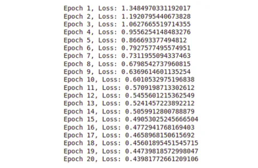
Conclusion
In conclusion, JAX is a powerful library for numerical computing and machine learning that offers many advantages over NumPy. It provides automatic differentiation, auto-vectorization, and JIT, which makes it easy to compute the complex equations used in ML models. Further it also supports CPU and GPU acceleration, allowing for faster computations on large datasets.
Reference
-
- Jax: High Performance Array Computing – Documentation.